In machine learning and statistics, loss functions are used to measure the performance of a machine learning algorithms. Loss functions are typically optimized to increase the predictive performance of the model. One loss function that you may be familiar with is the sum squared error. In linear regression, the sum squared error is minimized and is used to calculate the coefficients for the linear equation over the training data set.
The sum squared error can be derived by using minimizing the KL divergence between the the true but unknown theoretical distribution and our machine learning model. The KL divergence can be thought of as the dissimilarity measure between two distribution and is minimized to maximize the similarity between the theoretical distribution and our machine learning model.
Let  be the true but unknown theoretical distribution and
  be the machine learning model. For instance, lets assume it is a linear regression model.
Then using the equation for the KL divergence.
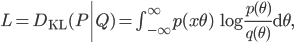

We can calculate  by sampling from the true distribution
  .
.
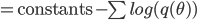
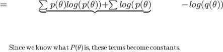
Since we are trying to minimizing the KL divergence, the constants be ignored and the equations becomes:
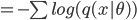
Now going back to the linear regression example. Let's assume that  , then the loglikehood is now:
= 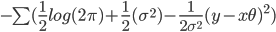
Since our goal is to minimize the KL divergence, to maximize the similarity between the empirical and theoretical distribution we can safely ignore the constants. And since we assume that the distribution is a normal distribution with variance 1, we can substitute in one for  .
.
The loss equation then becomes:
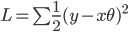
which is the equation for the sum squared error.